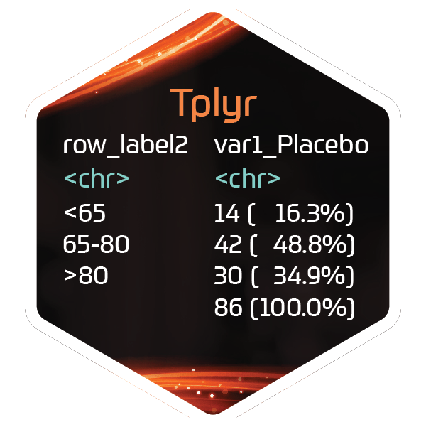
Adding a total row creates an additional observation in the count summary that presents the total counts (i.e. the n's that are summarized). The format of the total row will be formatted in the same way as the other count strings.
Arguments
- e
A
count_layerobject- fmt
An f_str object used to format the total row. If none is provided, display is based on the layer formatting.
- count_missings
Whether or not to ignore the named arguments passed in `set_count_missing()` when calculating counts total row. This is useful if you need to exclude/include the missing counts in your total row. Defaults to TRUE meaning total row will not ignore any values.
- sort_value
The value that will appear in the ordering column for total rows. This must be a numeric value.
Details
Totals are calculated using all grouping variables, including treat_var and
cols from the table level. If by variables are included, the grouping of the
total and the application of denominators becomes ambiguous. You will be
warned specifically if a percent is included in the format. To rectify this,
use set_denoms_by(), and the grouping of add_total_row() will
be updated accordingly.
Note that when using add_total_row() with set_pop_data(), you
should call add_total_row() AFTER calling set_pop_data(),
otherwise there is potential for unexpected behaivior with treatment groups.
Examples
# Load in Pipe
library(magrittr)

tplyr_table(mtcars, gear) %>%
  add_layer(
    group_count(cyl) %>%
      add_total_row(f_str("xxxx", n))
   ) %>%
   build()
#> # A tibble: 4 × 6
#>   row_label1 var1_3        var1_4        var1_5      ord_layer_index ord_layer_1
#>   <chr>      <chr>         <chr>         <chr>                 <int>       <dbl>
#> 1 4          " 1 (  6.7%)" " 8 ( 66.7%)" " 2 ( 40.0…               1           1
#> 2 6          " 2 ( 13.3%)" " 4 ( 33.3%)" " 1 ( 20.0…               1           2
#> 3 8          "12 ( 80.0%)" " 0 (  0.0%)" " 2 ( 40.0…               1           3
#> 4 Total      "  15"        "  12"        "   5"                    1           4
