Slides

Workshop Goals

This workshop is not exhaustive but meant to be a first contact with the R programming language. We hope you leave the workshop able to say:

R isn’t scary!

We also hope to show you you can use R to do things with data you’re already familiar with, as well as clinical computations.

Object Types

Data Frames in R are like Datasets in SAS®. Data frames are made up of columns called vectors – treated like Variables in SAS® More data types exist, but we’ll focus on data frames

Basic Variable Types

Numeric

Character

Boolean

a	b	c
1	a	TRUE
2	b	TRUE
3	c	FALSE

Assigning Variables

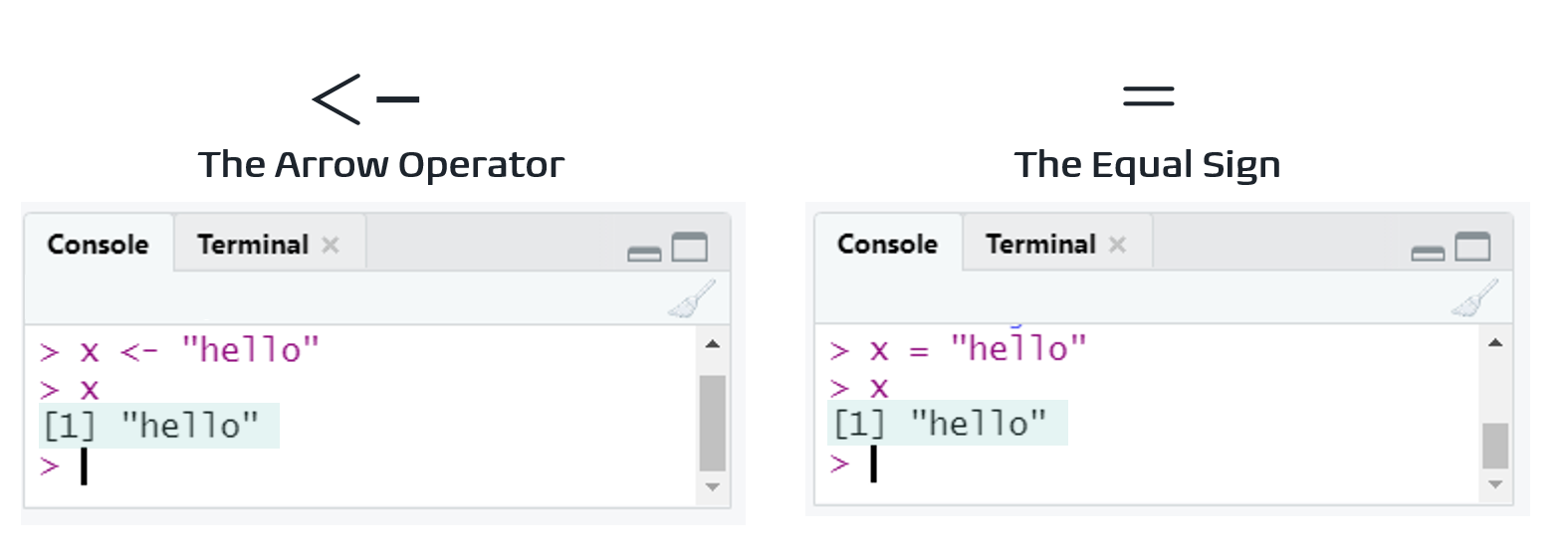
These two methods yield the same results, but the convention is to use <-. Learn more here

Testing Equality

Operator	Meaning	Example
<-	assign	x <- y
==	equal to	x == y
!=	not equal to	x != y
<	less than	x < y
<=	less than or equal to	x <= y
>	greater than	x > y
>=	greater than or equal to	x >= y

Arithmetic Operators

operator	Meaning	Example	Result
+	addition	1 + 1 == 2	2
-	subtraction	1 -1 == 0	0
/	division	6/3 == 2	2
*	multiplication	2 * 3 == 6	6
^ or **	exponentiation	3 ** 2 or 3 ^ 2	9
%%	modulus	6%%5	1
%%	integer division	7 %% 2	3

A Couple More

Operator	Meaning	Example
&	and	x & y
|	or	x | y
!	not	!x
%in%	in	x %in% y

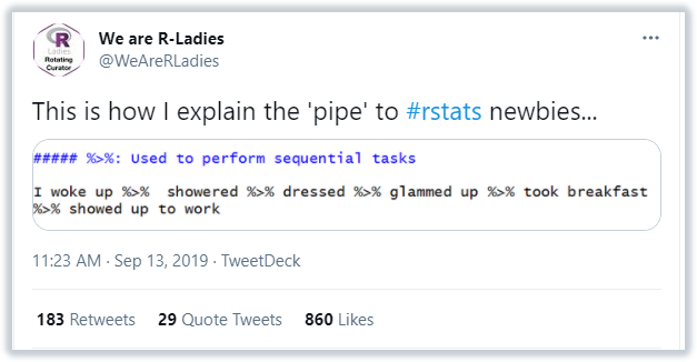
The Pipe %>% Operator

The pipe, %>%, is used to create a pipeline of functions and can be read as “and then”

What are packages?

Packagers are collections of functions and tools to expand the capabilities of R. You can import a package with: library(package_name)

What is the tidyverse?

The tidyverse is an opinionated collection of R packages designed for data science. All packages share an underlying design philosophy, grammar, and data structures.

Install the complete tidyverse with: install.packages("tidyverse")

Keep:

We can keep only the columns a and b from the original dat:

a	b	c
X	5	15
X	10	20
Y	2	12
Y	7	17

With the code:

dat %>%
  select(a,b)

a	b
X	5
X	10
Y	2
Y	7

Drop

We can drop column c, choosing everything but column c:

a	b	c
X	5	15
X	10	20
Y	2	12
Y	7	17

By using the code:

dat %>%
  select(-c)

a	b
X	5
X	10
Y	2
Y	7

Sub-setting by rows (where)

We can subset dat where f >= 5

a	b	c
X	5	15
X	10	20
Y	2	12
Y	7	17

Using the following code:

dat %>%
  filter(b>=5)

a	b
X	5
X	10
Y	7

Rename

We can use R’s rename function to rename columns a and b to groups and values. Given this starting data frame:

a	b	c
X	5	15
X	10	20
Y	2	12
Y	7	17

We can use the code:

dat %>%
  rename(
    groups = a,
    values = b
  )

groups	values	c
X	5	15
X	10	20
Y	2	12
Y	7	17

Sorting data

Compared to SAS®, you don’t have to sort a lot of the time!

When do I sort? - Presentation - Order dependent operations (i.e. baseline flag) - Don’t need it for grouping

For instance, if we want to sort our data frame by column b:

a	b	c
X	5	15
X	10	20
Y	2	12
Y	7	17

We can use the arrange function on column b

dat %>%
  arrange(b)

a	b	c
Y	2	12
X	5	15
Y	7	17
X	10	20

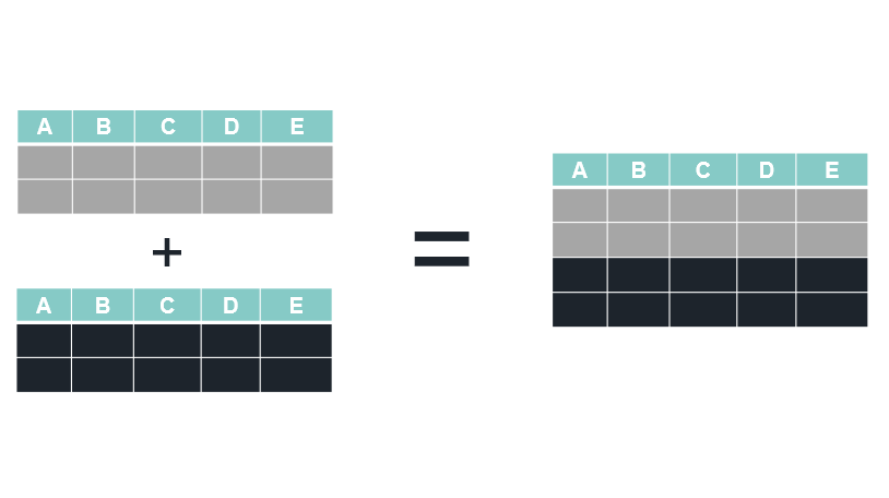
set AKA bind_rows

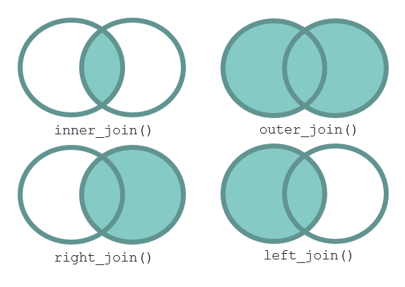
merge AKA *_join

Adding/editing a variable

We can use the mutate function to create new columns using the data from existing columns. For instance we can create a new column c by adding 10 to column b. We can also use the mutate function to or modify existing columns in place. For example, rather than create a new column, we can overwrite column a adding - before and after each entry.

Original Data

a	b
X	5
X	10
Y	2
Y	7

Using the following code:

dat %>%
  mutate(
    c = b + 10,
    a = paste0("-", a, "-")
)

a	b	c
-X-	5	15
-X-	10	20
-Y-	2	12
-Y-	7	17

if_else logic

We can use if_else within a mutate to create new columns based on another column. For instance, we can create a categorical column of High and Low values based on column b:

a	b
X	5
X	10
Y	2
Y	7

We can use this code:

dat %>%
  mutate(
    level = if_else(b > 5,
                    "High",
                    "Low")
    )

a	b	level
X	5	Low
X	10	High
Y	2	Low
Y	7	High

But what if we want another, Medium category for values greater than 3 but less than 7?

a	b
X	5
X	10
Y	2
Y	7

If we were to use an if_else statement that would require nesting

dat %>%
  mutate(
    level = if_else(b < 3, "Low",
                    if_else(b < 8, "Mid",  "High"))
    )

But this is really hard to read! Lucky for us we can use the case_when function.

The structure of case_when can be read as:

• Left side of ~ True/False or something that evaluates to True/False

• Right side of ~ Value to return

dat %>%
  mutate(
    level = case_when(
      b < 3 ~ "Low",
      b < 8 ~ "Mid",
      TRUE ~ "High"
    )
  )

a	b	level
X	5	Medium
X	10	High
Y	2	Low
Y	7	Medium

rowwise vs column operators

dat %>%
  mutate(
    c = mean(c(a,b))
  )
#

a	b	c
5	5	6.375
16	10	6.375
3	2	6.375
3	7	6.375

dat %>%
  rowwise() %>%
  mutate(
    c = mean(c(a,b))
  )

a	b	c
5	5	5.0
16	10	13.0
3	2	2.5
3	7	5.0

Descriptive Statistics

a	b
X	5
X	10
Y	2
Y	7

dat %>%
  summarize(
    mean = mean(b),
    sd = sd(b),
    min = min(b),
    max = max(b)
  )

mean	sd	min	max
6	3.36	2	10

Grouped Descriptive Statistics

a	b
X	5
X	10
Y	2
Y	7

dat %>%
  group_by(a) %>%
  summarize(
    mean = mean(b),
    sd = sd(b),
    min = min(b),
    max = max(b)
  )

a	mean	sd	min	max
X	7.5	3.53	5	10
Y	4.5	3.53	2	7

Counting

Option 1

a	b
X	dog
X	cat
X	rabbit
Y	rabbit
Y	rabbit

dat %>% 
  group_by(b) %>% 
  summarize( 
    n = n() 
  )

a	b
1	dog
1	cat
3	rabbit

Option 2

a	b
X	dog
X	cat
X	rabbit
Y	rabbit
Y	rabbit

dat %>% 
  count(b)

a	b
1	dog
1	cat
3	rabbit

Grouped Option 1

a	b
X	dog
X	cat
X	rabbit
Y	rabbit
Y	rabbit

dat %>% 
  group_by(a, b) %>% 
  summarize( 
    n = n() 
  )

a	b
1	dog
1	cat
3	rabbit

Other Options

In the course we also showcase 2 other ways to achieve the same goal. The first is using group_by and count

dat %>%
  group_by(a) %>% 
  count(b)

or with even shorter code, calling count on both columns we’d like to group by:

dat %>%
  count(a, b)