End-to-End Example • clinify

This vignette walks through a program in a fuller context. Here we’re going to create a simple demographics table.

First we’ll start by preparing the data. We’ll use our other package {Tplyr} to take care of the summaries.

library(clinify)
library(Tplyr)
library(dplyr)
#> 
#> Attaching package: 'dplyr'
#> The following objects are masked from 'package:stats':
#> 
#>     filter, lag
#> The following objects are masked from 'package:base':
#> 
#>     intersect, setdiff, setequal, union

tplyr_adsl <- tplyr_adsl |>
  mutate(
    SEX = recode(SEX, M = "Male", F = "Female"),
    RACE = factor(
      RACE,
      c(
        "AMERICAN INDIAN OR ALASKA NATIVE",
        "ASIAN",
        "BLACK OR AFRICAN AMERICAN",
        "NATIVE HAWAIIN OR OTHER PACIFIC ISLANDER",
        "WHITE",
        "MULTIPLE"
      )
    )
  )

t <- tplyr_table(tplyr_adsl, TRT01P) |>
  add_layer(
    group_count(SEX, by = "Sex n (%)") |>
      set_missing_count(f_str("xx", n), Missing = NA, denom_ignore = TRUE)
  ) |>
  add_layer(
    group_desc(AGE, by = "Age (Years)")
  ) |>
  add_layer(
    group_count(AGEGR1, by = "Age Categories n (%)") |>
      set_missing_count(f_str("xx", n), Missing = NA, denom_ignore = TRUE)
  ) |>
  add_layer(
    group_count(RACE, by = "Race n (%)") |>
      set_missing_count(f_str("xx", n), Missing = NA, denom_ignore = TRUE) |>
      set_order_count_method("byfactor")
  ) |>
  add_layer(
    group_count(ETHNIC, by = "Ethnicity n (%)") |>
      set_missing_count(f_str("xx", n), Missing = NA, denom_ignore = TRUE)
  ) |>
  add_layer(
    group_desc(HEIGHTBL, by = "Height at Baseline")
  ) |>
  add_layer(
    group_desc(WEIGHTBL, by = "Weight at Baseline")
  )

# Apply some conditional formatting for blanking out 0's.
dat <- build(t) |>
  mutate(
    across(
      starts_with("var"),
      ~ if_else(
        ord_layer_index %in% c(1, 3:5),
        apply_conditional_format(
          string = .,
          format_group = 2,
          condition = x == 0,
          replacement = ""
        ),
        .
      )
    )
  )

# Sort all the row values out, add row masks and breaks
dat <- dat |>
  arrange(ord_layer_index, ord_layer_1, ord_layer_2) |>
  apply_row_masks() |>
  select(
    starts_with("row_label"),
    var1_Placebo,
    `var1_Xanomeline Low Dose`,
    `var1_Xanomeline High Dose`,
    ord_layer_index
  )

# Grab the header Ns for column header help
header_n <- t$header_n$n
names(header_n) <- t$header_n$TRT01P

Great - our data are presentation ready now. Using {clinify} we’ll get everything ready. Looking at some of these sections:

We use clin_auto_page() to let Word figure out page breaks for us.
Column headers are set using clin_column_headers(). We grabbed our header N’s from {Tplyr} and inserted them here.
We want our headers and parts of the body center aligned. Remember, we can use {flextable} functions directly on the clintable to do this.
Column widths are set using clin_col_widths() by using a proportion of the total desired table width.
Lastly we’ll add our titles and footnotes. We’re putting current and total pages in the top right of our titles. Given the default styling functions in {clinify}, which you can override yourself, page numbers are auto detected by using the strings {PAGE} and {NUMPAGES}.

ct <- clintable(dat) |>
  # Use group changes to let Word naturally split pages
  clin_auto_page("ord_layer_index", drop = TRUE) |>
  # Add padding to changes within the group
  # By using `notempty`, paging groups are determined by populated
  # values of `row_label1`
  clin_group_pad('row_label1', when = "notempty") |>
  # Assign column headers with spanning rows
  clin_column_headers(
    row_label1 = "",
    row_label2 = "",
    var1_Placebo = sprintf("Placebo\n(N=%s)", header_n["Placebo"]),
    `var1_Xanomeline Low Dose` = c(
      "Xanomeline",
      sprintf("Low Dose\n(N=%s)", header_n["Xanomeline Low Dose"])
    ),
    `var1_Xanomeline High Dose` = c(
      "Xanomeline",
      sprintf("High Dose\n(N=%s)", header_n["Xanomeline High Dose"])
    )
  ) |>
  # Use flextable functions directly to set all of the alignment
  flextable::align(align = "center", part = "header") |>
  flextable::align(
    j = c(
      "var1_Placebo",
      "var1_Xanomeline Low Dose",
      "var1_Xanomeline High Dose"
    ),
    align = "center"
  ) |>
  # Set column widths as proportion of the total document width
  clin_col_widths(
    row_label1 = .17,
    row_label2 = .3,
    var1_Placebo = .176,
    `var1_Xanomeline Low Dose` = .176,
    `var1_Xanomeline High Dose` = .176
  ) |>
  # Add titles here is using new_header_footer to allow flextable functions
  # to customize the titles block
  clin_add_titles(
    list(
      # We'll add tools to automate paging
      c("Protocol: CDISCPILOT01", "Page {PAGE} of {NUMPAGES}"),
      c("Table 14-2.01"),
      c("Summary of Demographic and Baseline Characteristics")
    )
  ) |>
  clin_add_footnotes(
    list(
      c(
        "Source: /my/file/path.R",
        format(Sys.time(), "%H:%M %A, %B %d, %Y")
      )
    )
  )

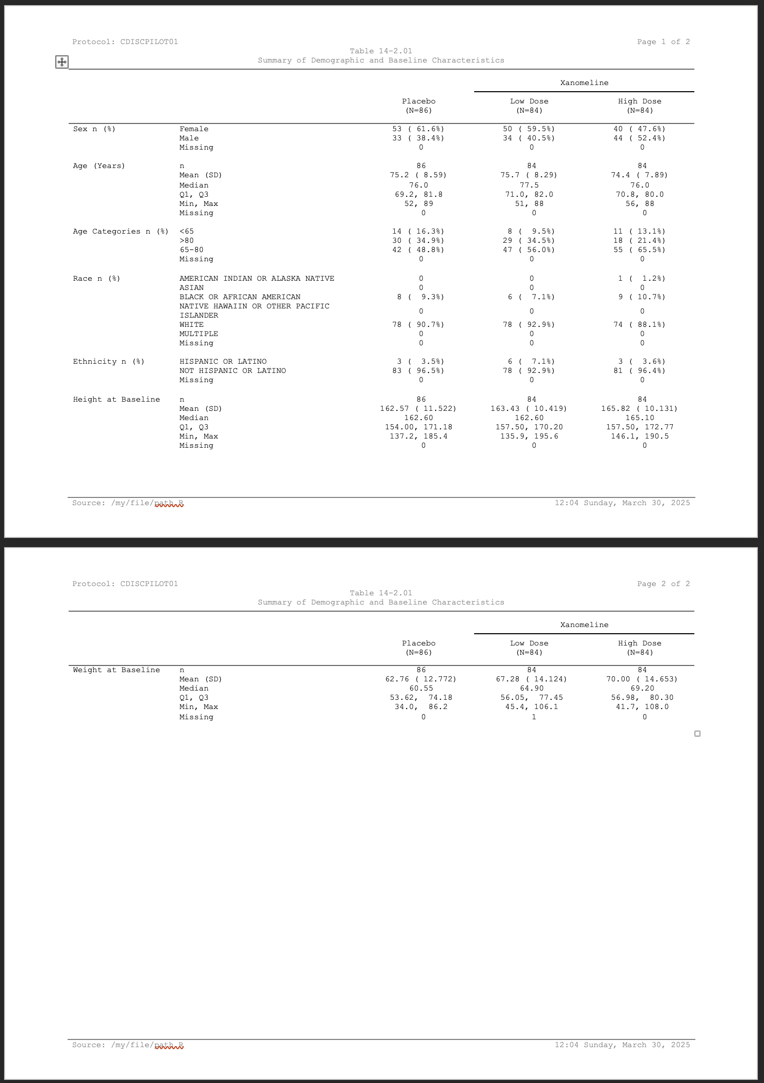
print(ct)

Protocol: CDISCPILOT01	Page of
Table 14-2.01
Summary of Demographic and Baseline Characteristics

			Xanomeline	Xanomeline
		Placebo (N=86)	Low Dose (N=84)	High Dose (N=84)
Sex n (%)	Female	53 ( 61.6%)	50 ( 59.5%)	40 ( 47.6%)
	Male	33 ( 38.4%)	34 ( 40.5%)	44 ( 52.4%)
	Missing	0	0	0
Age (Years)	n	86	84	84
	Mean (SD)	75.2 ( 8.59)	75.7 ( 8.29)	74.4 ( 7.89)
	Median	76.0	77.5	76.0
	Q1, Q3	69.2, 81.8	71.0, 82.0	70.8, 80.0
	Min, Max	52, 89	51, 88	56, 88
	Missing	0	0	0
Age Categories n (%)	<65	14 ( 16.3%)	8 ( 9.5%)	11 ( 13.1%)
	>80	30 ( 34.9%)	29 ( 34.5%)	18 ( 21.4%)
	65-80	42 ( 48.8%)	47 ( 56.0%)	55 ( 65.5%)
	Missing	0	0	0
Race n (%)	AMERICAN INDIAN OR ALASKA NATIVE	0	0	1 ( 1.2%)
	ASIAN	0	0	0

Source: /my/file/path.R

14:08 Tuesday, June 10, 2025

With everything ready to go, we can write our table out to its destination using write_clindoc().

write_clindoc(ct, "demo_table.docx")